This post describes how open source tools can be combined to ingest, store, and visualise thousands of real-time messages per minute - for less than the price of a coffee each month. The data source is Network Rail’s Train Movement feed [1], used here as a surrogate for Internet-of-Things (IoT) device telemetry. The focus is on raw message throughput, storage efficiency, and operational observability rather than interpreting the train movements themselves.
The following dashboard provides a snapshot of the pipeline after 9 days of continuous operation.
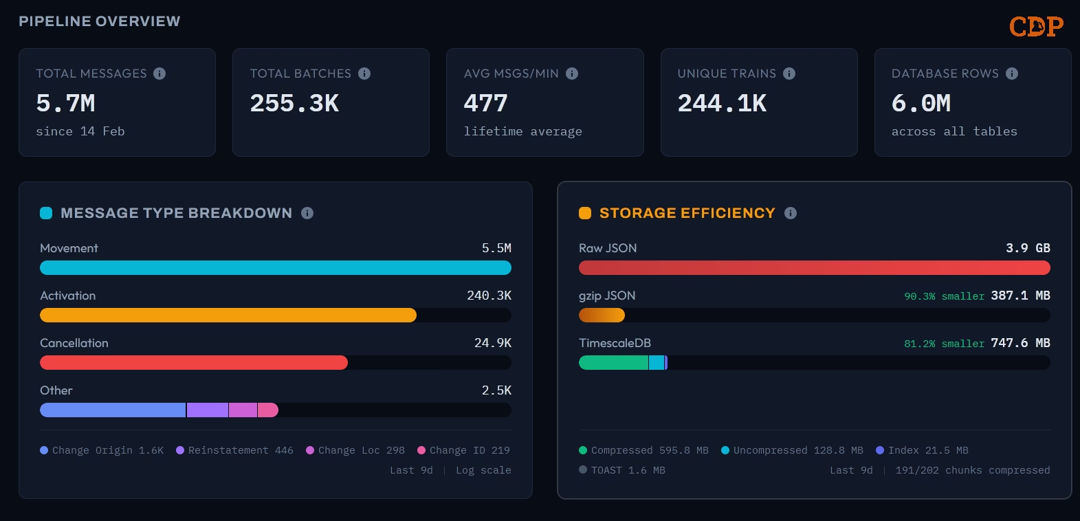
Pipeline overview showing 5.7 million messages ingested since 14 February across 255,000 Kafka batches
The headline numbers: 5.7 million messages processed at an average of 477 per minute, covering 244,000 unique trains, stored in 6 million database rows. The raw JSON would consume 3.9 GB; TimescaleDB [2] compression reduces this to 748 MB, an 81% reduction, with 191 of 202 chunks compressed. Using gzip as a comparison, the same data compresses to 387 MB (90% reduction), but without any of the query capabilities that a database provides.
The entire pipeline of ingestion, processing, storage, and web dashboard runs comfortably on a single virtual machine costing under £5 per month on providers like Hetzner [3], including 9 months of storage. On major cloud providers like Azure, the compute alone is under £5 per month (excluding storage). The point is not that production workloads should run on minimal infrastructure indefinitely, but that real-time data pipelines need not start with expensive managed services.
Introduction
The assumption that real-time data ingestion requires significant infrastructure investment is widespread. Conversations in enterprise IT departments often begin with managed stream processing platforms, dedicated clusters, and monthly bills measured in thousands. This assumption is rarely challenged because the tooling landscape has evolved around it: vendor documentation, reference architectures, and conference talks all reinforce the narrative.
An alternative exists. The PostgreSQL [4] ecosystem - specifically TimescaleDB for time series workloads - combined with lightweight stream processors like Logstash, Redpanda Connect etc and container orchestration through Podman [5] Quadlets, provides a capable and cost-effective stack for many real-time data use cases. A previous post on this blog, Cracking Compression, examined the storage and query characteristics of TimescaleDB using Formula 1 telemetry data. This post extends that analysis into a live, continuously running pipeline.
The data source is the Network Rail (NWR) Train Movement feed, a stream of messages from the TRUST (Train Running Under System TOPS) system that reports train activations, movements, cancellations, and other events across the UK rail network. These messages arrive via a managed Kafka broker as batched JSON documents, typically every 5 seconds, at rates of several hundred messages per minute. This feed exhibits the characteristics common to IoT telemetry: high frequency, semi-structured payloads, variable batch sizes, and a natural time series orientation.
Pipeline Architecture
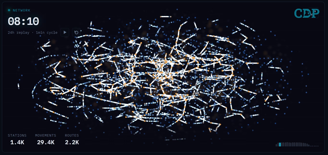
The architecture follows a deliberate pattern: a single stream processor consumes from the upstream broker, captures batch-level metrics as a side effect of ingestion, unpacks individual messages, and inserts them into a time series database. A web dashboard provides operational observability. A second data flow constructs a network graph from the movement messages, powering the animated visualisation shown at the top of this post.

Each Kafka message contains a batch of TRUST messages, typically between 10 and 30 individual events. Redpanda Connect acts as the Kafka consumer, using a branch processor to capture the raw byte size, gzip-compressed byte size, and message count of each batch before unpacking. These batch-level metrics are written to a dedicated batch_metrics hypertable, providing the storage efficiency comparison without adding per-message overhead to the ingestion path.
After metrics capture, the batch is unpacked into individual messages, key fields are extracted (timestamp, message type, train ID, location), and the messages are inserted into TimescaleDB in batches of 100 or every 5 seconds, whichever comes first. The entire pipeline runs as rootless Podman containers orchestrated by Systemd Quadlets on Ubuntu Server 24.04, ensuring the services restart automatically after reboots.
Pipeline Metrics
The pipeline overview captures the lifetime statistics. Over the first 9 days of operation, the system ingested 5.7 million individual messages delivered in 255,300 Kafka batches, maintaining a sustained average throughput of 477 messages per minute. The feed contained 244,100 unique train identifiers across 6.0 million database rows (the row count exceeds the message count because the batch_metrics table contributes additional rows).
Message Type Breakdown
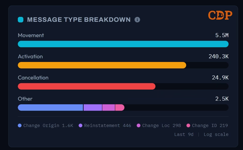
The message type distribution follows the expected pattern for the TRUST system. Movement messages (type 0003) dominate at 5.5 million - these represent a train arriving at or departing from a reporting point. Activations (240,300) and Cancellations (24,900) form the secondary tier, while the rarer operational types such as Change of Origin (1,600), Reinstatement (446), Change of Location (298), and Change of Identity (219) - appear in the long tail. The dashboard renders this on a logarithmic scale to make the distribution readable across four orders of magnitude.
Storage Efficiency
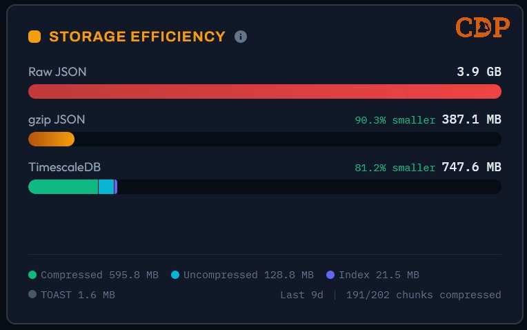
The three-way storage comparison is calculated from the batch-level metrics captured during ingestion. The 3.9 GB of raw JSON compresses to 387 MB using gzip (90.3% reduction). TimescaleDB stores the same data in 748 MB, with the segmented bar revealing the internal composition: 596 MB compressed data, 129 MB still awaiting compression, 22 MB of indexes, and 2 MB of TOAST (The Oversized-Attribute Storage Technique) overflow. The 191 of 202 chunks compressed reflects the compression policy - the most recent chunks remain uncompressed for fast writes, and are compressed by a background policy after aging beyond the retention threshold.
The gzip comparison is more storage-efficient in raw terms, but it’s a write-once format with no query capability. The TimescaleDB figure includes indexes, metadata, and the ability to run analytical queries directly against the compressed data.
Time series Analysis
The dashboard provides selectable time windows of 15 minutes, 1 hour, 24 hours, and 7 days, each with summary cards that contextualise the selected period. In the 1-hour view shown above, the system processed 35,400 messages in 1,500 batches at 590 messages per minute, covering 4,800 unique trains.
Message Throughput
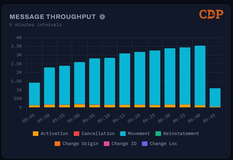
The message throughput chart displays a stacked bar at 5-minute intervals, decomposed by message type. The early morning period captured here shows the network ramping up: throughput climbs from around 1,200 messages at 05:45 to 3,500 by 06:35 as services begin running. Movement messages dominate each bar, with Activations forming a visible secondary layer. This is the same “awakening” pattern visible in the animated network graph, rendered here as a time series.
Batch Arrival Rate
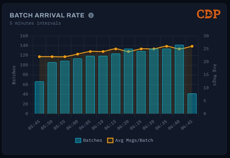
The batch arrival rate chart uses a dual-axis design: bars show the batch count per 5-minute interval (left axis), while a line traces the average messages per batch (right axis). The batch count roughly doubles over the hour - from 65 to 140 - as the upstream feed responds to increasing network activity. The average messages per batch, however, remains relatively stable around 20–25. This reveals an operational characteristic of the data source: Network Rail scales throughput by sending more frequent batches rather than larger ones.
Both charts leverage TimescaleDB’s time_bucket function through the batch_metrics hypertable, making these aggregations efficient even as the dataset grows. A previous post on this blog, Cracking Compression, examined the query performance characteristics of these time-bucket functions in detail.
Network Visualisation
The network visualisation is the hero element of the dashboard. It replays 24 hours of train movement data compressed into a 1-minute animation cycle, showing how the UK rail network builds from near-silence in the early hours to full activity during the day.
The graph is a force-directed layout using D3.js force simulation, seeded from geographic coordinates but optimised for topological clarity over geographic accuracy, following the design philosophy of the London Underground map. The dense cluster of locations in and around London, which would occupy a tiny fraction of a geographic projection, is spread into a readable arrangement by the force simulation.
Nodes represent STANOX (Station Number) reporting locations - a broader concept than passenger stations. STANOX codes identify any location where a train movement is reported: stations, junctions, sidings, depots, freight terminals, and passing points. Of the 1,500 locations active in the visualisation, many are junctions and operational locations that passengers would never see. Their size scales with cumulative traffic - major junctions and terminus stations grow visibly larger as the animation progresses. The colour temperature shifts from cool blue (inactive or low-traffic) to warm amber (high-traffic), creating an automatic visual hierarchy. Edges represent observed train movements between consecutive reporting points, rendered with a glow effect using a dual-canvas technique - one canvas for sharp detail, another with CSS blur for the ambient bloom.
The data feeding this visualisation is pre-computed using TimescaleDB continuous aggregates, refreshed hourly. The animation itself runs entirely on the client using HTML5 Canvas at 60fps, with no WebSocket or live data connection - it simply replays the last 24 hours of pre-aggregated data fetched via a standard API call.
Setup
The pipeline runs as four containers on a single host. The following table summarises the key components:
| Concern | Technology | Notes |
|---|---|---|
| Stream Processing | Logstash / Redpanda | Kafka consumer, Bloblang transforms, batched SQL output |
| Time series Storage | TimescaleDB (PostgreSQL 16) | Hypertables, compression, continuous aggregates |
| Web Dashboard | SvelteKit (Svelte 5) + Bun | Metric cards, Chart.js visualisations, D3 network graph |
| Documentation | VitePress | Static site served alongside the dashboard |
| Container Runtime | Podman (rootless) | Systemd Quadlets for lifecycle management |
| Reverse Proxy | Traefik | TLS termination and routing (cloud deployment) |
| Host OS | Ubuntu Server 24.04 LTS | Headless, systemd lingering enabled |
The Kafka connection uses SASL_SSL authentication against a managed Confluent Cloud broker. Credentials for the Network Rail data feeds are obtained from the Rail Data Marketplace, which provides access to a range of real-time and historic rail data under the Open Government Licence.
Conclusion
The combination of a modern stream ingestion tool, TimescaleDB, and Podman demonstrates that real-time data pipelines can be both capable and economical. The pipeline ingests hundreds of messages per minute, compresses storage by 81%, powers analytical queries through time series hyperfunctions, and drives a network visualisation, all on infrastructure costing less than £5 per month.
This is not an argument against managed services or the lakehouse pattern. Both serve genuine needs at scale. The argument is that many real-time data use cases, particularly in IoT telemetry, operational monitoring, and sensor data, can start with a fraction of the assumed infrastructure cost and scale only when demand warrants it. The PostgreSQL ecosystem, and TimescaleDB in particular, provides a foundation where storage efficiency and analytical capability are not competing concerns but complementary ones.
The animated network graph that opens this post was built from the same data, using the same database, on the same infrastructure. That is the unreasonable effectiveness of choosing the right tools.
Version History
2026-04-10- Revised punctuation and heading levels for consistency.2026-03-01- Original
Attribution
The train movement data used in this project is sourced from Network Rail via the TRUST (Train Running Under System TOPS) system, accessed through a managed Kafka broker. This data is published under the Open Government Licence v3.0.
Our use of this data is not endorsed by Network Rail. We gratefully acknowledge Network Rail for making this data available to support innovation and research.
Images used in this post have been generated using multiple Machine Learning (or Artificial Intelligence) models and subsequently modified by the author.
Where ever possible these have been identified with the following symbol:

The text has been reviewed using Large Language Models for spelling, grammar, and word choice; however, the content, analysis, and conclusions are entirely the author’s own.
References
Citation
@online{miah2026,
  author = {Miah, Ashraf},
  title = {Ingesting a {Nation’s} {Railway:} {Real-time} {Data}
    {Pipelines} for {Under} £5 a {Month}},
  date = {2026-03-01},
  url = {https://blog.curiodata.pro/posts/20-nwr-pipeline/},
  langid = {en}
}